While this is one useful way to view the global economic picture, it’s not the only way. Today’s visualization, which comes to us from HowMuch.net, is similar in that it also uses a Voronoi diagram to display the composition of the world economy by GDP. However, by adjusting data for purchasing power parity (PPP), it produces a very different view of how global productivity breaks down.
What is PPP?
Purchasing power parity, or PPP, is an economic theory that can be applied to adjust the prices of goods in a given market. In essence, instead of using current market rates for prices (such as in nominal data), PPP tries to more accurately account for differences in the cost of living between countries – especially in places where labor and goods are far cheaper. When applied to GDP measurements, PPP can help provide a more accurate picture of actual productivity. For example, a taxi ride in Bolivia may be far cheaper than one in New York City, even though it is the same service provided over the same distance. Applying PPP to GDP figures can help correct for these types of differences.
Ranked: Economies by GDP (PPP)
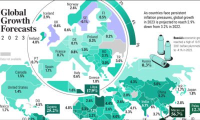
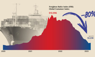
After adjusting for PPP, how does the composition of the global economy change from the nominal numbers? Below are the 15 largest economies by GDP (PPP), as well as how their ranking changed from the previous chart, which used nominal data. Using GDP (PPP), the world economy is worth $136.5 trillion in current international U.S. dollars. What changed the most from the nominal ranking? With PPP, you can see Indonesia ($3.5 trillion) jumps up the ranking by nine spots to become the #7 ranked economy. Likewise, Turkey ($2.4 trillion) and India ($10.5 trillion) both climb the ranking by six and four spots respectively. China also switches with the U.S., to become the world’s largest economy. On the flipside, it is often the more developed economies with strong currencies that see a drop in their rankings. After adjusting for PPP, the United States, Japan, Germany, France, Italy, South Korea, Spain, and the U.K. all slip from their previous positions. For more on GDP (PPP), see the projections for the world’s largest 10 economies in 2030 that we published earlier this year. on Last year, stock and bond returns tumbled after the Federal Reserve hiked interest rates at the fastest speed in 40 years. It was the first time in decades that both asset classes posted negative annual investment returns in tandem. Over four decades, this has happened 2.4% of the time across any 12-month rolling period. To look at how various stock and bond asset allocations have performed over history—and their broader correlations—the above graphic charts their best, worst, and average returns, using data from Vanguard.
How Has Asset Allocation Impacted Returns?
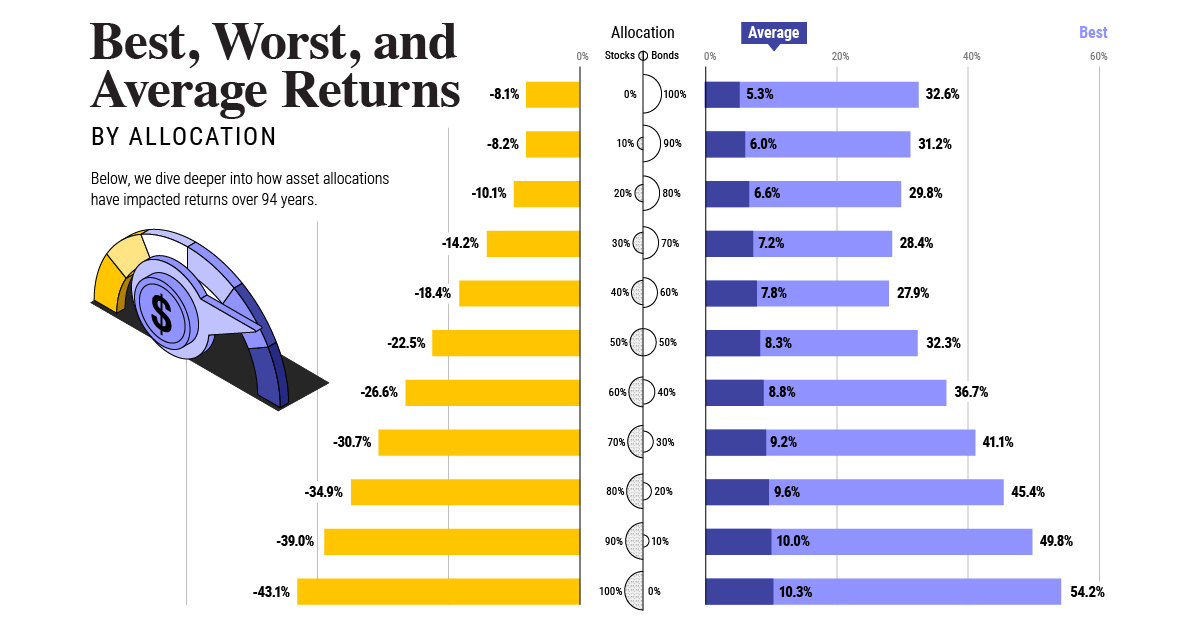
Based on data between 1926 and 2019, the table below looks at the spectrum of market returns of different asset allocations:
We can see that a portfolio made entirely of stocks returned 10.3% on average, the highest across all asset allocations. Of course, this came with wider return variance, hitting an annual low of -43% and a high of 54%.
A traditional 60/40 portfolio—which has lost its luster in recent years as low interest rates have led to lower bond returns—saw an average historical return of 8.8%. As interest rates have climbed in recent years, this may widen its appeal once again as bond returns may rise.
Meanwhile, a 100% bond portfolio averaged 5.3% in annual returns over the period. Bonds typically serve as a hedge against portfolio losses thanks to their typically negative historical correlation to stocks.
A Closer Look at Historical Correlations
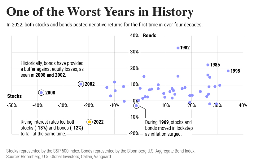
To understand how 2022 was an outlier in terms of asset correlations we can look at the graphic below:
The last time stocks and bonds moved together in a negative direction was in 1969. At the time, inflation was accelerating and the Fed was hiking interest rates to cool rising costs. In fact, historically, when inflation surges, stocks and bonds have often moved in similar directions. Underscoring this divergence is real interest rate volatility. When real interest rates are a driving force in the market, as we have seen in the last year, it hurts both stock and bond returns. This is because higher interest rates can reduce the future cash flows of these investments. Adding another layer is the level of risk appetite among investors. When the economic outlook is uncertain and interest rate volatility is high, investors are more likely to take risk off their portfolios and demand higher returns for taking on higher risk. This can push down equity and bond prices. On the other hand, if the economic outlook is positive, investors may be willing to take on more risk, in turn potentially boosting equity prices.
Current Investment Returns in Context
Today, financial markets are seeing sharp swings as the ripple effects of higher interest rates are sinking in. For investors, historical data provides insight on long-term asset allocation trends. Over the last century, cycles of high interest rates have come and gone. Both equity and bond investment returns have been resilient for investors who stay the course.